Datahader.Networks 绘制bundling flow
详细文档参见 https://datashader.org/user_guide/Networks.html
我们曾经介绍了绘制普通流的方式,实际上仅仅是基于贝塞尔曲线做了插值,绘制了类似于“飞机航线”的流线。使用简单的arcgis插件,也可以绘制很不错直观的流图,比如下面我画的中国人口流动图:
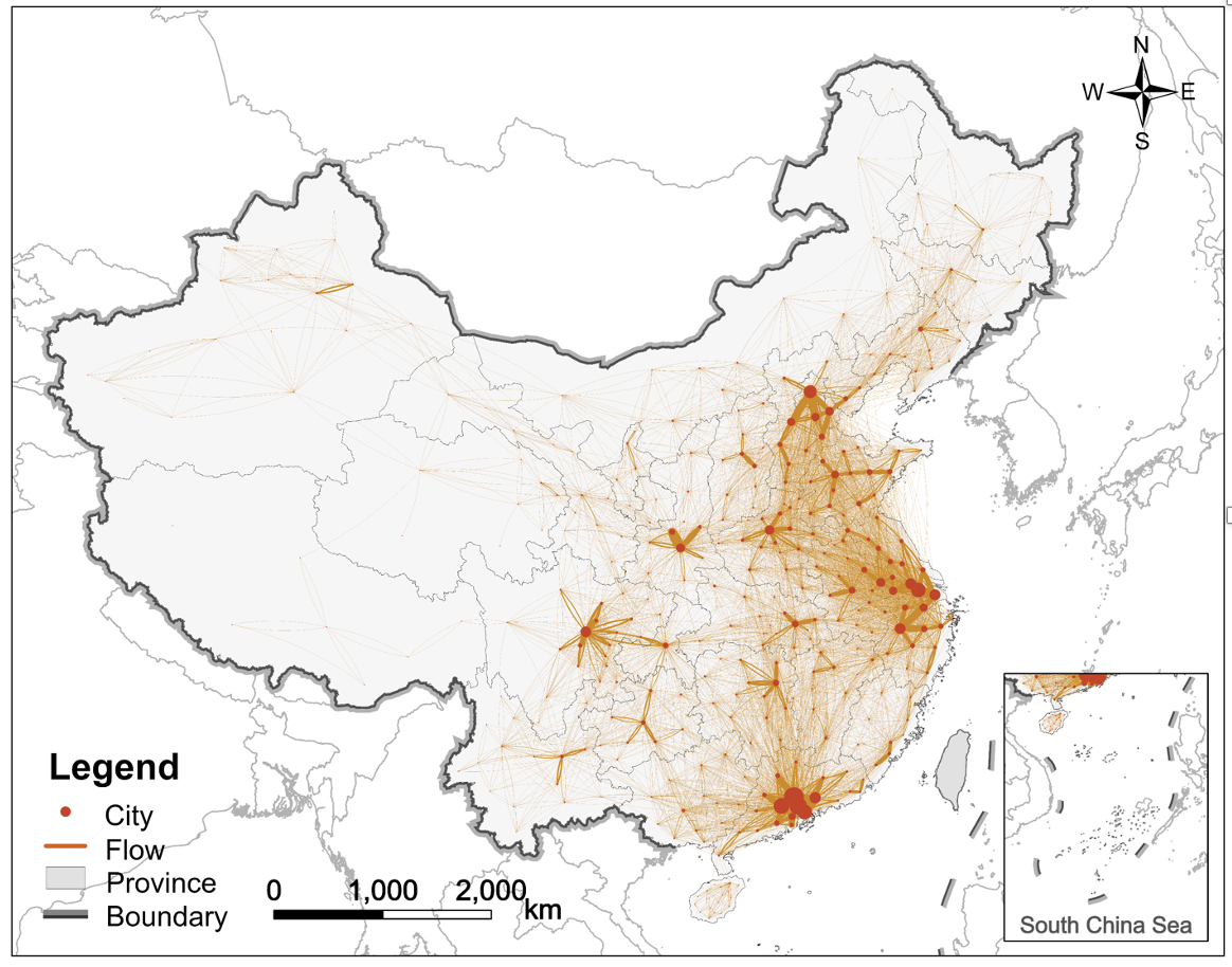
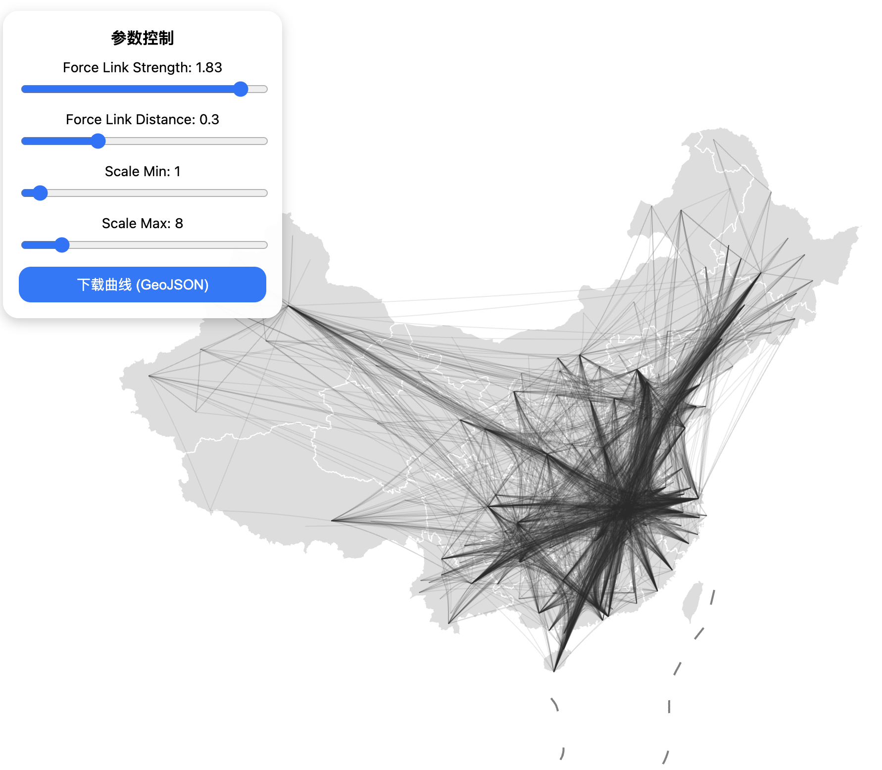
但是这种流绘制方式虽然最为直观、表达最为准确,但有时候(特别是边权差异不大的时候)像进了盘丝洞,从图上无法提炼出太多的信息,因此,甲方要求我对小红书上一个博主绘制的具有聚集效应的流图进行复现,我先试了js库d3:
1 | function generateSegments(nodes, links) { |
大概实现了下面的场景:
不过这种绘制方法仍然无法达到类似的效果,遂抛弃之,找到了该博主处理流数据的库:datashader,接下来我们详细讲讲如何利用datashader.Networks进行绘制,先看看user guide中对该部分的简介:
The point and line-segment plotting provided by Datashader can be put together in different ways to visualize specific types of data. For instance, network graph data, i.e., networks of nodes connected by edges, can very naturally be represented by points and lines. Here we will show examples of using Datashader’s graph-specific plotting tools, focusing on how to visualize very large graphs while allowing any portion of the rendering pipeline to replaced with components suitable for specific problems.
Datashader 使用 Hammer et al. (2009) 提出的 “Force-Directed Edge Bundling (FDEB)” 算法的改进版,让相似或空间上邻近的边“靠拢”成平滑的流线(bundles),既保持结构关系,又提升可读性。
具体来说,对于每条边,他们会被拆分为多个小段(segments),每个 segment 是一个可移动的控制点。每个控制点会受到几种力的作用:
-
- 内部张力 (Tension)
-
- 相似边吸引力 (Attractive force)
-
- 带宽控制 (Bandwidth)
通过多次迭代,方法使得带宽逐次变小,使得流互相靠近,形成束状结构。
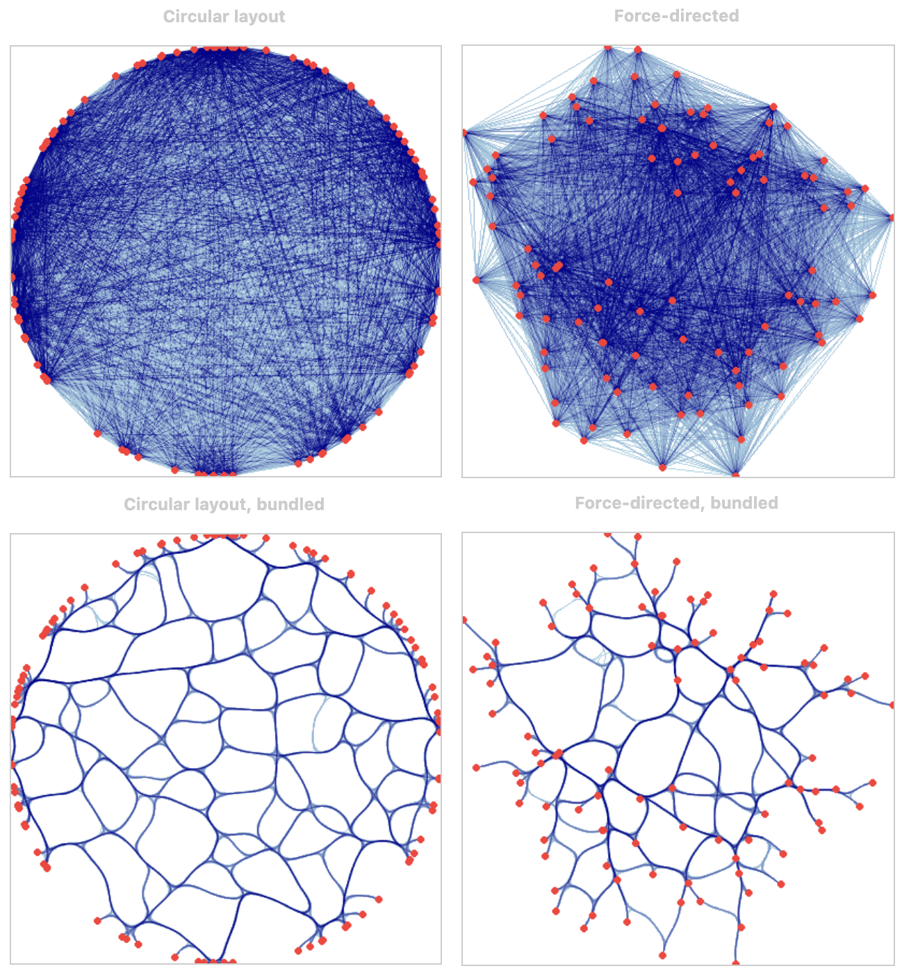
我们来复现一下user guide提供的示例代码
导入包
1 | import math |
随机生成边与节点
1 | np.random.seed(0) |
生成布局与定义一些绘制函数
1 | cvsopts = dict(plot_height=400, plot_width=400) |
绘制:
1 | cd = circular |
还是挺方便的。接下来我们使用自己的数据进行绘制。必要的数据包括node(包含name与xy坐标)和edge(包含代表od的source和target,可自行选择是否加上weight)。
导入包:
1 | import pandas as pd |
加载数据,并映射一下字段名到其要求的值,并且投影坐标以绘制。这里有一个非常坑的要点:
node 的 index(pandas.dataframe的index)才是和 edge 的 source 与 target 匹配的 key ,而不是 name 字段。
1 | china_edge = pd.read_csv("/Users/fangtianyao/Desktop/其他/flowdata/edge_1.csv") |
调用hammer_bundle计算:
1 | bundled_edges = hammer_bundle(layout, edges, decay=decay, initial_bandwidth=bw) |
这里的 decay 和 bw 是两个0-1的参数,这里我们先分别取0.5。
计算得到的 bundled_edges 是一个包含所有扭曲过后的边的所有构成点的df,每条边的点之间用一个空行相隔。打印给你看看。
| x | y | weight | |
|---|---|---|---|
| 1301138 | 1.257390e+07 | 2.951534e+06 | 7.0 |
| 1301139 | 1.258085e+07 | 2.914048e+06 | 7.0 |
| 1301140 | 1.258971e+07 | 2.877599e+06 | 7.0 |
| 1301141 | 1.264494e+07 | 2.852891e+06 | 7.0 |
| 1301142 | NaN | NaN | NaN |
为了绘制,我们使用该数据创建 GeoDataFrame:
1 | lines = [] |
我们用这个数据绘制流在地图上:
1 | import geopandas as gpd |
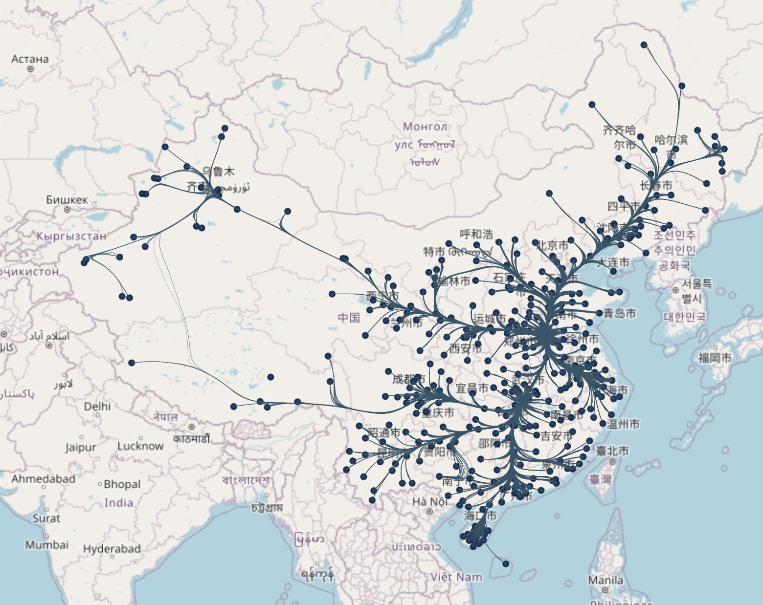
为了比较不同 decay 和 bw 参数组合的效果,我做了一个小组合测试,读者可以自己进行测试,亦可以参考下user guide里面基于随机数据做的测试。
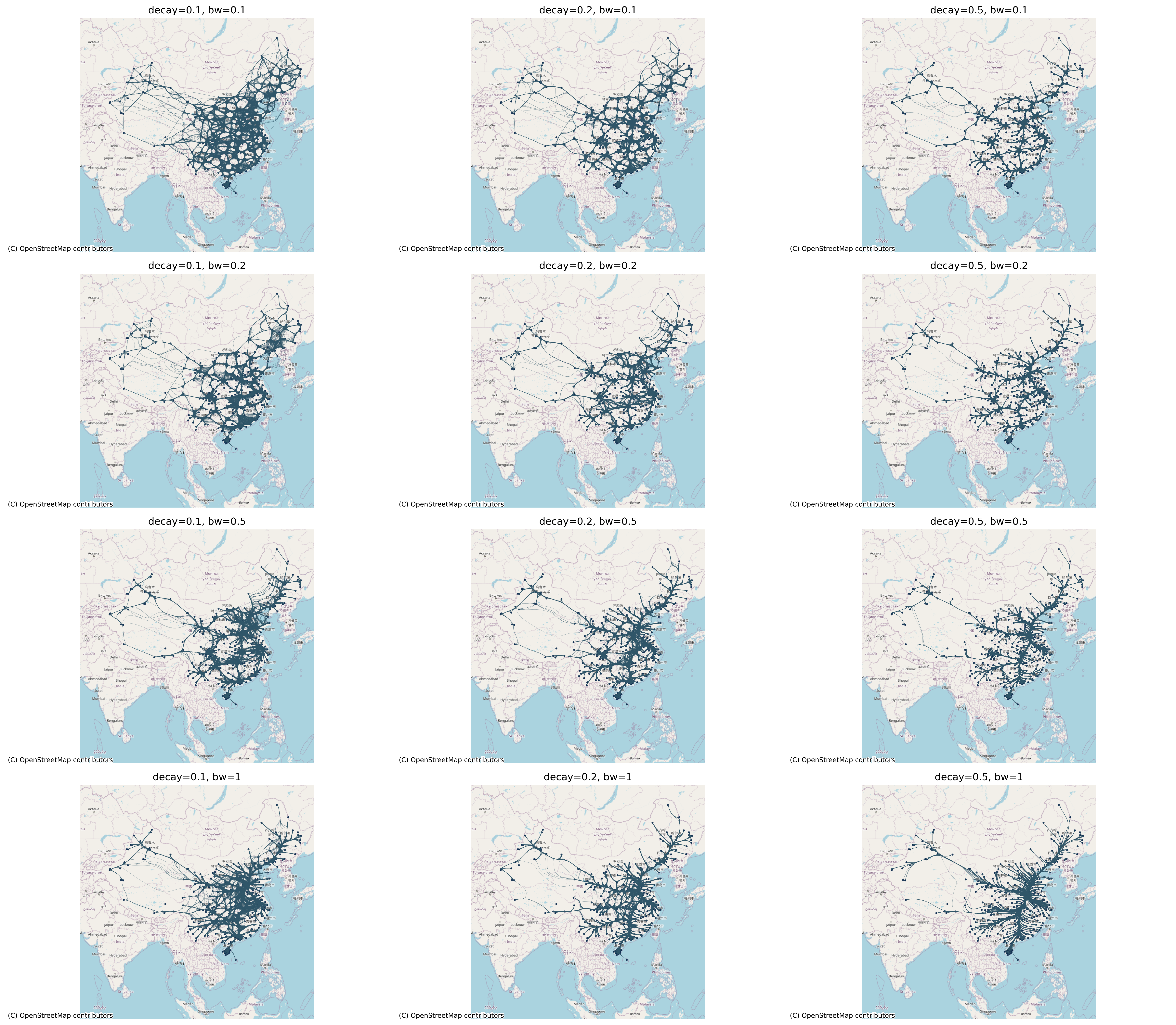
还是不错的吧😌
最后给出封装好的函数,该函数用于对空间网络数据执行基于 Hammer 算法 的边捆绑(Edge Bundling)操作,以减少边的视觉交叉并增强整体结构的空间可读性。
输入参数
• edge_path (str):边数据文件路径,要求为 CSV 格式,包含源节点、目标节点及权重等字段。
• node_path (str):节点数据文件路径,要求为 CSV 格式,包含节点唯一标识及经纬度坐标字段。
• nodes_id_col (str):节点文件中表示节点唯一编号的列名,默认 “node_id” 务必是int类型!!!。
• node_lon_col (str):节点经度列名,默认 “lon”。
• node_lat_col (str):节点纬度列名,默认 “lat”。
• edge_source_col (str):边文件中表示起点节点的列名,默认 “source” 和上面的node_id匹配,务必是int类型!!!。
• edge_target_col (str):边文件中表示终点节点的列名,默认 “target” 和上面的node_id匹配,务必是int类型!!!。
• weight_col (str):边文件中表示权重(如流量、强度)的列名,默认 “weight”。
• decay (float):Hammer 算法的衰减参数,控制边的收敛速度(0–1之间)。
• bw (float):初始带宽参数,控制捆绑的紧密程度(0–1之间)。
• input_crs (str):输入数据的坐标参考系,默认 “EPSG:4326”(WGS84)。
• output (bool):是否输出文件,默认 True。
• output_format (Literal[“geojson”, “shp”]):输出文件格式,默认 “geojson”。
• output_path (Optional[str]):输出文件保存路径,若为 None,则仅返回结果不保存。
输出结果
• 返回值 (geopandas.GeoDataFrame):
函数返回一个包含边捆绑后几何结果的 GeoDataFrame,其属性包括原始边的全部字段及对应的空间几何 (LineString)。结果的坐标参考系为 “EPSG:4326”,可直接用于 GIS 可视化或空间分析。
若设置 output=True,则函数还会在指定路径下导出相应的 GeoJSON 或 Shapefile 文件。
1 | import pandas as pd |
1 | def perform_edge_bundling( |